Chapter 10 : Matrix inverse

1. Analogy

In elementary algebra, the solution of the following equation is said to be the multiplicative inverse :

$$\begin{equation} ax = 1 \end{equation}$$

The solution of $(1)$ is $\frac{1}{a}$, which is also written $a^{-1}$.

In linear algebra, the equivalent equation to $(1)$ is :

$$\begin{equation} AA^{-1} = I \end{equation}$$

In $(2)$, $I$ is the so-called identity matrix. It contains $1$’s on its diagonal and $0$’s everywhere else, as follows : $\left( \begin{smallmatrix} 1 & \cdots & 0 \\ \vdots & \phantom{/} 1 & \vdots \\ 0 & \cdots & 1 \end{smallmatrix} \right)$.

2. Calculation

The inverse matrix of $A=\left(
\begin{smallmatrix}
a_{1,1} & \cdots & a_{1,n} \\
\vdots & \cdots & \phantom{1}\vdots \\
a_{n,1} & \cdots & a_{n,n}
\end{smallmatrix}
\right)$ is obtained by dividing the transpose of the cofactor matrix, noted $C^{T}$, by the determinant of $A$ :

In $(3)$ there are two new concepts. First, the matrix of cofactors (or comatrix), second the transpose of a matrix.

Let’s first explain how to transpose a matrix. To transpose a matrix, convert its rows into columns.

Example I

Let $A=\left( \begin{smallmatrix} -5 & 0 \\ -8 & -1 \end{smallmatrix} \right)$. Let’s compute its transpose.

$$\begin{equation} \left( \begin{smallmatrix} -5 & 0 \\ -8 & -1 \end{smallmatrix} \right)^T = \left( \begin{smallmatrix} -5 & -8 \\ 0 & -1 \end{smallmatrix} \right) \end{equation}$$

Let’s now look at the cofactor matrix. The cofactor $c_{i,j}$ of $a_{i,j}$ is defined as follows :

In $(5)$, $D_{i,j}$ is the determinant of $A$ without the row $\textbf{i}$ and without the column $\textbf{j}$.

Example II

Let $A=\left( \begin{smallmatrix} -5 & 0 \\ -8 & -1 \end{smallmatrix} \right)$. Let’s compute $D_{1,2}$ of $A$.

$$D_{\color{orangered}{1},\color{orangered}{2}} = \begin{vmatrix} \enclose{horizontalstrike}{-5} & \enclose{horizontalstrike}{\color{orangered}{0}} \\ -8 & \enclose{horizontalstrike}{-1} \end{vmatrix} = \begin{vmatrix} -8 \end{vmatrix} = -8$$

Example III

Let $A=\left( \begin{smallmatrix} 2 & 1 \\ 5 & -1 \end{smallmatrix} \right)$. Let’s compute its inverse.

First, let’s compute its determinant :

$$\begin{equation} \det(A) = \begin{vmatrix} 2 & 1 \\ 5 & -1 \end{vmatrix} = 2\cdot -1-5\cdot 1=-7 \end{equation}$$

Second, let’s compute the cofactor matrix :

$$\begin{equation} C = \left( \begin{array}{} (-1)^{(1+1)}\begin{vmatrix} -1 \\ \end{vmatrix} & (-1)^{(1+2)}\begin{vmatrix} 5 \\ \end{vmatrix} \\ (-1)^{(2+1)}\begin{vmatrix} 1 \\ \end{vmatrix} & (-1)^{(2+2)}\begin{vmatrix} 2 \\ \end{vmatrix} \end{array} \right) = \left( \begin{array}{} -1 & -5 \\ -1 & 2 \end{array} \right) \end{equation}$$

Third, let’s compute the transpose of $C$ and thus get the inverse of $A$:

3. Inverse function

More generally, the matrix inverse can be seen as an inverse function.

In analysis, an inverse function, noted $f^{-1}$, maps the images back to the elements in the original set, as Figure 10.1 illustrates.

It turns out that a function has an inverse only if it is bijective.

Figure 10.1 : inverse function (wikipedia)

Figure 10.2 : bijection

A bijection is a function having a special property.
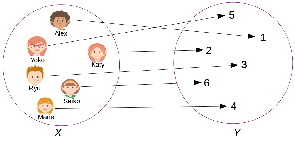
Any element from the starting set is associated, under the function, to one single element in the target set and vice versa. Figure 10.2 shows this property.

Example IV

Let $t$ :

$$\begin{equation} t \colon \, \mathbb{R}^2 \to \mathbb{R}^2 \\ \left( \begin{smallmatrix} x_1 \\ x_2 \end{smallmatrix} \right) \mapsto \left( \begin{smallmatrix} 2 & 1 \\ -6 & -3 \end{smallmatrix} \right) \left( \begin{smallmatrix} x_1 \\ x_2 \end{smallmatrix} \right) \end{equation}$$

$t$ is not bijective since many $\vec{x}$ are associated to $\vec{y}=\left( \begin{smallmatrix} 0 \\ 0 \end{smallmatrix} \right)$.
Indeed, by decomposing, $x_1
\left( \begin{smallmatrix} 2 \\ -6 \end{smallmatrix} \right) + x_2 \left( \begin{smallmatrix} 1 \\-3 \end{smallmatrix} \right) =
\left( \begin{smallmatrix} 0 \\ 0 \end{smallmatrix} \right)$ has infinitely many solutions because the vectors are linearly dependent.

Wrap-up