Chapter 12 : Diagonalization

1. Analogy

Let’s assume that we’d like do a numerical processing in the best suited base on this purpose.

Let’s have an example : we’d like to divide an even number by $2$. It turns out that the base 2 is the best suited base for doing that. Indeed a simple shift from left to right does that processing.

We have the three following steps :

1. Change of basis (from decimal to binary)
2. We do the processing in that new base (shift)
3. Change of basis (from binary to decimal)

Example I

Let’s divide $208$ by $16$.

Let’s proceed the above steps discussed :

1. Conversion of $208$ into the base 2 : 11010000
2. 1st shift : 01101000. 2nd shift : 00110100. 3rd shift : 00011010. 4th shift : 00001101
3. Conversion of 00001101 into the decimal base : $13$

2. Calculation

A diagonalizable matrix $A$ is decomposed as follows :

In $(1)$ $P$ is the eigenvectors matrix of $A$ and $D$ the eigenvalues matrix of $A$.

In our analogy of above, the calculation of $A\vec{x}$ would be the numerical processing. We then have in $(1)$, from right to left :

1. Conversion of $\vec{x}$ in a new basis, becoming $\vec{x}’$
2. Processing the linear transformation in the new basis : $D\vec{x}’=\vec{y}’$
3. Conversion of $\vec{y}’$ in the starting basis, becoming $\vec{y}$

Example II

Let $A=\left( \begin{smallmatrix} 2 & 1 \\ 3 & 4 \end{smallmatrix} \right)$. Let’s diagonalize $A$.

We determined the eigenvectors of $A$ in the dedicated chapter (let $\beta=1$).

Then $P=\left( \begin{smallmatrix} 1 & 1 \\ -1 & 3 \end{smallmatrix} \right)$ and $P^{-1}= \frac{1}{4}\left( \begin{smallmatrix} 3 & -1 \\ 1 & 1 \end{smallmatrix} \right).$ The matrix of the eigenvalues is : $D=\left( \begin{smallmatrix} 1 & 0 \\ 0 & 5 \end{smallmatrix} \right)$.

The diagonalization of $A$ is thus :

3. But more concretely ?

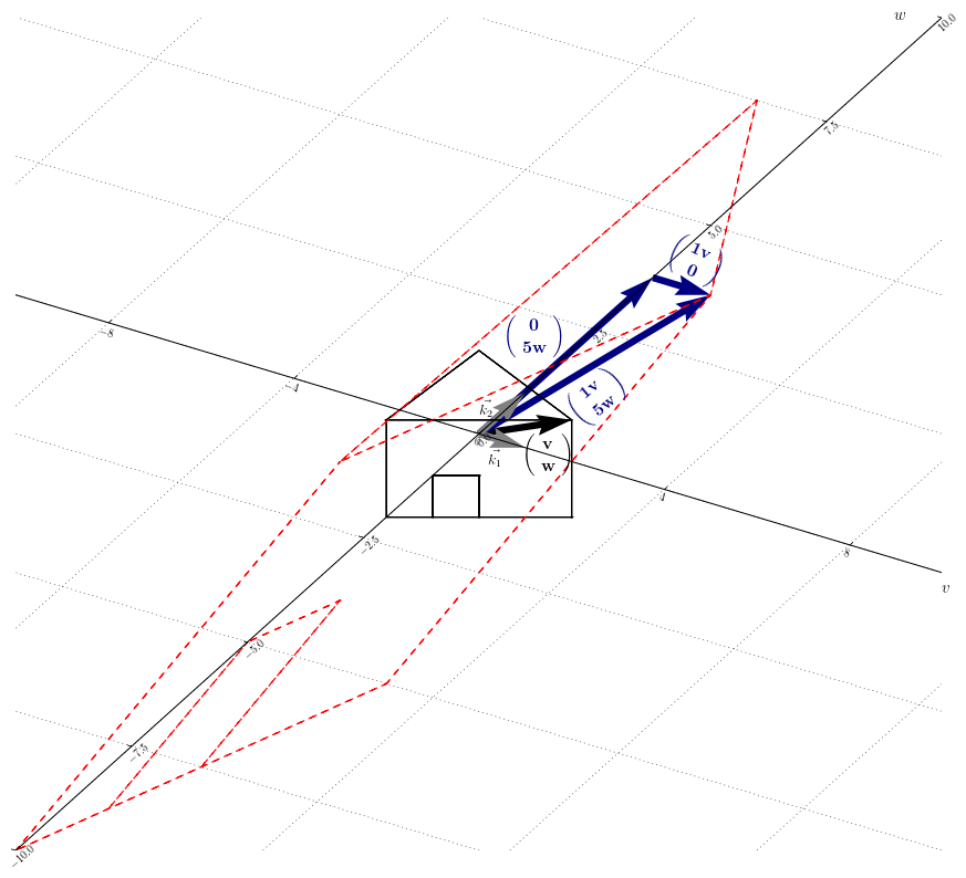
The point of the diagonalization is to proceed the linear transformation in a more suited basis. This new basis is composed of the eigenvectors and turns to be a new axis system.

This reduces the calculation amount, since in the new basis, $\vec{y}’$ is obtained by multiplying by a factor $\lambda_i$ the components of $\vec{x}$ for each axis independently from one another. Figure 12.1 shows the linear transformation of the example II in the new basis : $D \underbrace{ \left( \begin{smallmatrix} v \\ w \end{smallmatrix} \right) }_{\vec{x}’}
= \underbrace{\left( \begin{smallmatrix} 1v \\ 5w \end{smallmatrix} \right)
}_{\vec{y}’}$.

Figure 12.1 : linear transformation in a new basis

Recapitulation